Excel is the “standard” of the spreadsheet programs and is simply indispensable in daily work. With Excel, Microsoft has created one of the most ingenious programs that can help you immensely with a wide variety of work. That’s how it works
connecting cells
one of the helpful functions if you try to center an overview of several columns in a complex Excel table. Therefore it makes sense to combine these cells into one large cell . We would like to show you how this ” Connect cells ” function works in Excel in this short Excel tutorial .
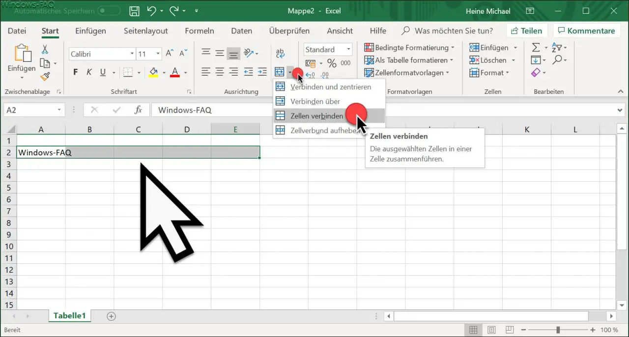
We would like to show you this function using an example. In the figure below you can see a column heading with the content ” Windows FAQ “. We want to center this text as the heading of columns A2 – E2.

To do this, you first mark the Excel cells that are to be connected to a cell. In our example you can see the marking of columns A2 – E2. Then you have to click on the small icon below ” Check “. We have marked this with a small red dot in the illustration.
Then the “Connect” context menu opens , in which you have 4 options. In our case, you choose the function
connecting cells
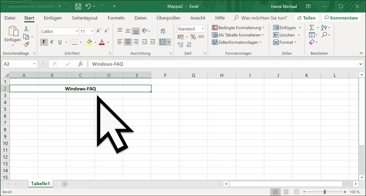
Excel then dissolves the borders of the selected cells and combines the selected cells into one large cell . You can see what this looks like in the figure below.

As you can see, the dividing lines between the columns have disappeared and the cell is now larger than the surrounding cells. Now you can, for example, bring the overview into the center of the connected cell using the ” Center ” function.
If you want to dissolve the connected Excel cells , you only need to click in the connected cell and the function
Remove cell network
to confirm.
You can find more tips and tricks around Microsoft Excel here:
– Display Outlook, Word, Excel and PowerPoint in dark design (Dark Mode) – Easily
restore unsaved Excel files
– Create a continuous diagram of an Excel table with missing values
– Simply import CSV files into Excel